netCDF 101

Joffrey JOUMAA

August 22, 2023

What’s a netCDF file?

NetCDF (Network Common Data Form) is a set of software libraries and self-describing, machine-independent data formats that support the creation, access, and sharing of array-oriented scientific data. The project homepage¹ is hosted by the Unidata program at the University Corporation for Atmospheric Research (UCAR). They are also the chief source of netCDF software, standards development, updates, etc. The format is an open standard. NetCDF Classic and 64-bit Offset Format are an international standard of the Open Geospatial Consortium.²

– Wikipedia

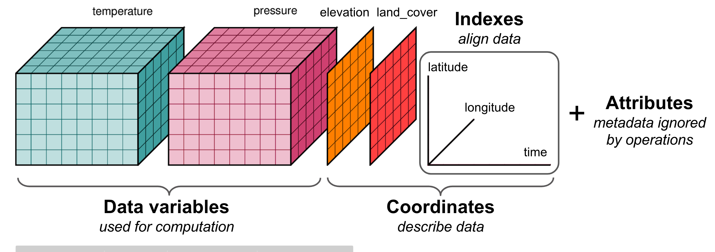
The way I see a netCDF file is that it’s a matrix that usually contains environmental data across time and location, plus extra information (called metadata) such as where does the dataset comes from, or its resolution.

Here is an example³ of the structure of a netCDF file containing information on temperature and pressure accross time for several location, but also on the elevation and the land cover

How to open it?

Super simple, using the tidync package! Let’s say you have a netcdf file called global-reanalysis-phy-001-031-grepv2-daily_1639765258612.nc, here is what you have to do to import this file:

# first load `tidync` package
library(tidync)

# then import your file
df_nc <- tidync("../inst/extdata/copernicus/global-reanalysis-phy-001-031-grepv2-daily_1639765258612.nc")

# flatten the multidimensional array
df <- df_nc %>%
  # extract NetCDF data as an expanded table
  hyper_tibble() %>%
  # not mandatory, but here is the code to convert to a data.table
  setDT()

# print the first 10 rows
df[sample(nrow(df), 10), ] %>%
  sable(
    caption = "First 10 rows of the flatten netCDF file",
    digits = 2
  )

First 10 rows of the flatten netCDF file

uo_cglo	uo_glor	vo_oras	uo_foam	vo_glor	uo_oras	vo_cglo	vo_foam	longitude	latitude	depth	time
0.05	0.20	-0.12	0.11	-0.06	0.10	-0.02	-0.13	-140.00	51.00	0.51	25148
0.06	0.04	0.04	0.10	0.03	0.01	-0.04	-0.21	-127.00	43.50	0.51	25161
-0.07	-0.17	-0.06	-0.23	-0.11	-0.17	-0.16	-0.08	-130.25	36.75	0.51	25400
0.03	-0.06	-0.03	-0.01	-0.12	0.01	0.05	-0.11	-131.75	27.75	0.51	25078
-0.03	-0.14	-0.08	0.00	0.01	-0.04	-0.09	-0.04	-156.25	30.00	0.51	25363
0.04	0.02	0.03	0.06	0.04	0.04	-0.02	-0.07	-136.00	35.50	0.51	25382
0.01	-0.01	0.11	0.00	-0.07	0.05	-0.02	-0.03	-152.75	48.25	0.51	25284
0.15	0.17	0.04	0.07	0.07	0.07	0.13	0.02	-149.25	28.25	0.51	25240
-0.02	-0.04	0.00	-0.08	-0.02	-0.04	-0.02	-0.05	-127.00	43.50	0.51	25314
0.11	0.16	-0.11	0.10	0.00	0.11	-0.08	-0.06	-160.50	40.75	0.51	25164

Now we can see that the time is not in a proper format. The first thing to do is to look into the metadata to see if we could find some kind of explanation. To do that, we’re going to use the ncmeta package, developped for this purpose.

# load ncmeta library
library(ncmeta)

# then we use the function nc_atts to access attributes of times
print(
  nc_atts(
    "../inst/extdata/copernicus/global-reanalysis-phy-001-031-grepv2-daily_1639765258612.nc",
    "time"
  ) %>%
    # we want information on the unit for time column
    dplyr::filter(name == "units") %>%
    pull(value)
)

## $units
## [1] "days since 1950-01-01 00:00:00"

The column time seems to be the number of days since 1950-01-01. Let’s use that information to format the time column in a proper way.

# convert time into a readable format
df[, time := as.Date(time, origin = as.Date("1950-01-01"))]

# print
df[sample(nrow(df), 10), ] %>%
  sable(
    caption = "First 10 rows of the flatten netCDF file, with reformat time column",
    digits = 2
  )

First 10 rows of the flatten netCDF file, with reformat time column

uo_cglo	uo_glor	vo_oras	uo_foam	vo_glor	uo_oras	vo_cglo	vo_foam	longitude	latitude	depth	time
-0.01	0.04	0.01	0.04	-0.08	-0.04	-0.01	0.02	-141.50	50.25	0.51	2019-01-02
0.02	0.11	0.03	0.10	0.04	0.00	0.08	0.06	-138.50	27.50	0.51	2018-07-25
0.03	0.01	-0.01	0.09	0.00	0.06	-0.02	-0.01	-143.50	29.00	0.51	2018-11-30
0.07	0.01	-0.02	-0.03	-0.03	0.00	-0.05	0.00	-133.50	41.00	0.51	2019-02-28
0.07	0.07	0.05	0.10	0.03	0.03	0.03	0.04	-154.00	52.75	0.51	2018-07-26
-0.02	-0.05	-0.04	-0.11	-0.07	-0.05	-0.06	0.00	-129.25	37.25	0.51	2019-06-07
0.01	0.09	0.00	0.00	0.01	-0.01	0.01	0.04	-152.50	44.75	0.51	2019-03-09
0.00	0.04	0.03	0.05	0.09	-0.04	0.04	0.07	-133.75	47.75	0.51	2018-05-07
-0.01	0.09	0.01	0.06	-0.04	0.04	0.01	-0.04	-139.00	51.75	0.51	2018-07-07
-0.07	0.08	0.01	0.13	-0.10	0.03	-0.06	-0.19	-127.00	28.75	0.51	2018-07-03

How to visualize it?

Well there are plenty of ways to display data within a netCDF. Here, we are only presenting one simple way to do it using ggplot2 and gganimate package.

# first let's calculate the velocity norm
df[, `:=`(
  vel_cglo = sqrt(uo_cglo^2 + vo_cglo^2),
  vel_oras = sqrt(uo_oras^2 + vo_oras^2),
  vel_foam = sqrt(uo_foam^2 + vo_foam^2),
  vel_glor = sqrt(uo_glor^2 + vo_glor^2),
  month = month(time),
  year = year(time)
)]

# average by month
df_summarize <- df[, .(
  vel_cglo = mean(vel_cglo, na.rm = T),
  vel_oras = mean(vel_oras, na.rm = T),
  vel_foam = mean(vel_foam, na.rm = T),
  vel_glor = mean(vel_glor, na.rm = T)
),
by = .(
  date = paste(year, "-", month),
  longitude,
  latitude
)
] %>%
  .[, time := .GRP, by = .(date)]

# data wrangling
dataPlot <- melt(df_summarize,
  id.vars = c("date", "longitude", "latitude", "time"),
  variable.name = "model"
)

# let's comput the ouput of all models
res_anim <- ggplot() +
  geom_raster(
    data = dataPlot,
    aes(x = longitude, y = latitude, fill = value),
    interpolate = TRUE
  ) +
  geom_sf(
    data = spData::world,
    col = 1,
    fill = "ivory"
  ) +
  coord_sf(xlim = c(-165, -115), ylim = c(25, 55)) +
  facet_wrap(. ~ model, ncol = 2) +
  theme_jjo() +
  theme(legend.position = "bottom") +
  labs(x = NULL, y = NULL) +
  scale_fill_gradientn(colours = oce::oceColors9A(120)) +
  labs(title = "Date: {df_summarize[,unique(date)][frame_time]}") +
  transition_time(time) +
  ease_aes("linear")

# let's print
animate(res_anim, height = 500, width = 500)

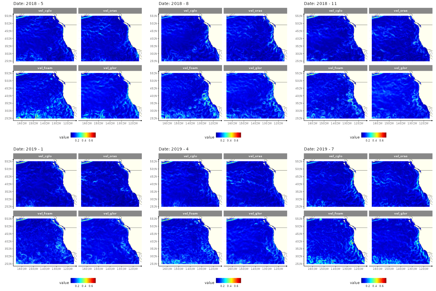
4 models of the current velocity in the North-East part of Pacific ocean

Four different GIFs, since there are four different models to get the SST: